I've never had a 3D printer before, but I've always known that I probably should. So when the new Monoprice Mini Delta 3D Printer was announced on Indiegogo I jumped in and got one of the early shipments for $159. This write-up is partly reminder for me about the steps I took to get it working, and partly to help anyone else just getting started with the Mini Delta. I do all of my work on Linux, so I can't say anything about setting it up under macOS or Windows.

I've printed a few copies of the test object (Maneki-neko) because both of my kids wanted one. I also printed a replacement zipper pull for my daughter's backpack just in time for her to start school. To test out some tiny prints, and further interest my kids, I printed a few simple rings for them (and one for me when I mistook diameter for radius). The most robotics-related thing I've printed is a pulley for some #6 ball chain. I'll be using that to make a simple X-Y pen plotter.

I didn't purchase any filament with the printer, so when it arrived I ran out to Fry's and picked up a 1 kg spool of yellow (my 1 year old was with me and he liked the yellow) Shaxon PLA (1.75mm diameter). I've had no problems with this filament, but have nothing to compare it with.

All in all, I love the Mini Delta. The build volume is not large, but I don't see that as a problem because if I actually tried to fill that volume I'd be printing for most of the day. And all the things I plan on printing are small mechanical components for my projects. For larger structural components I feel like laser cutting is the way to go. I did run into a few hiccups...

Issues encountered

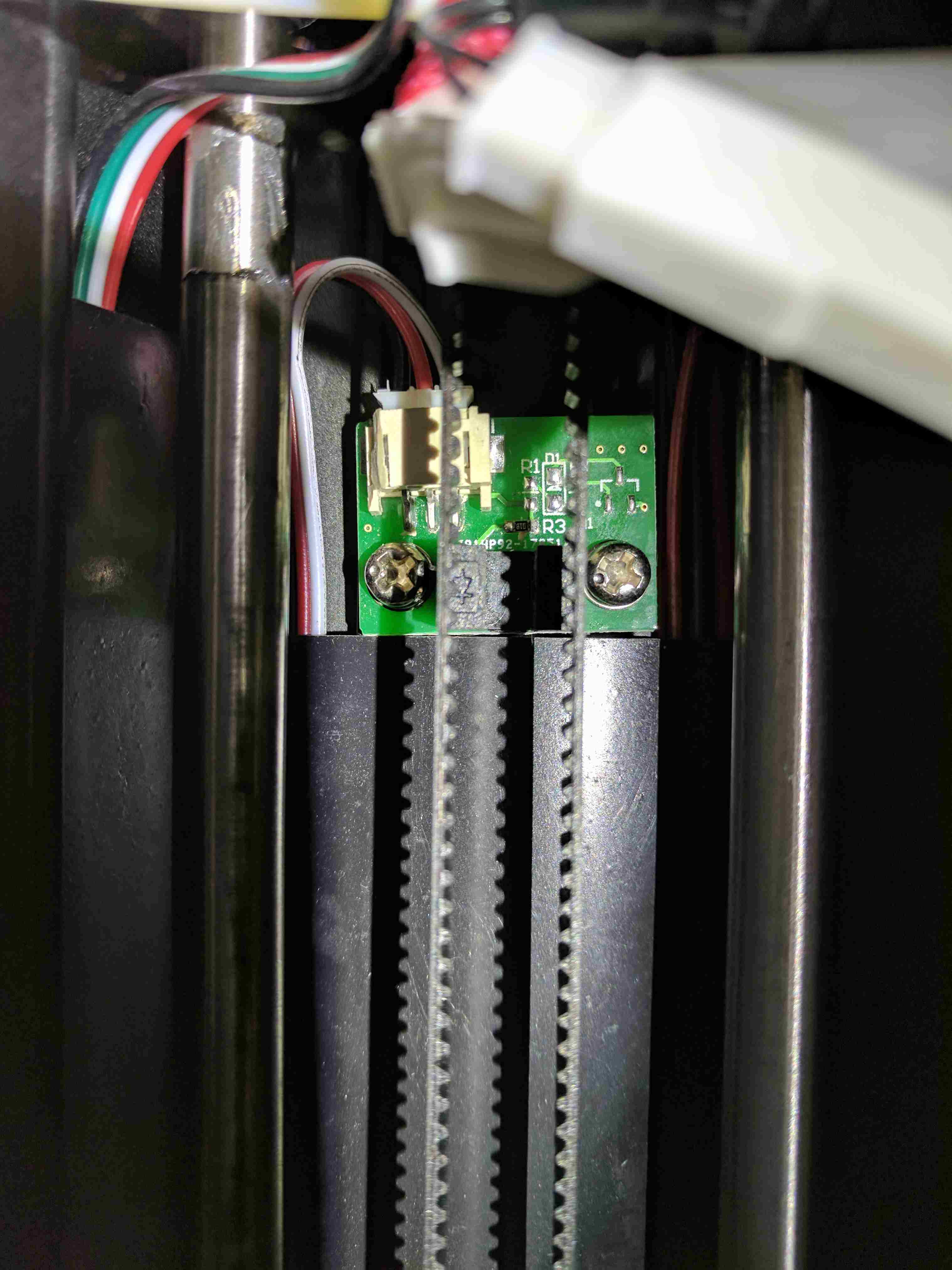
When I first unboxed and plugged in the machine I asked it to home its axes. While trying to home its print head, one of the three timing belt carriages got stuck at the top and made a nasty grinding noise, but managed to move back down, and then seemed fine. I should have investigated more at that time, but wanted to get to printing. So I started the sample print job that came on the SD card. Unfortunately, the sticking at the top of one of the carriages caused the machine to not quite know where the print head was, which made one side of the bed seem lower than it actually was, which caused the print head to scrape the bed while printing the initial raft. The first image below is of the damage to the print bed, pretty minimal actually, and it hasn't affected print adhesion. The second image is a picture of what I think is the culprit: the optical endstop sensor at the top of the column. If you look carefully at the three conductor connector, you can see that the header shroud is not symmetric, in fact the left side has been cut away, manually. I checked and this has been done to all three such connectors at the top of each column. If this manual step had not been done the bearing carriage would hit the header shroud and prevent the carriage from reaching the fully homed position. My guess is that this was a last minute change in parts or placement on the PCB, and this interference wasn't noticed until a few machines were manufactured. And it was likely much cheaper to have someone carve away the offending plastic than to remake the endstop boards. So, my guess is that this endstop header shroud was not fully clearing the carriage, resulting in a bind that caused the stepper controller to lose some steps, resulting in the hot end crash.

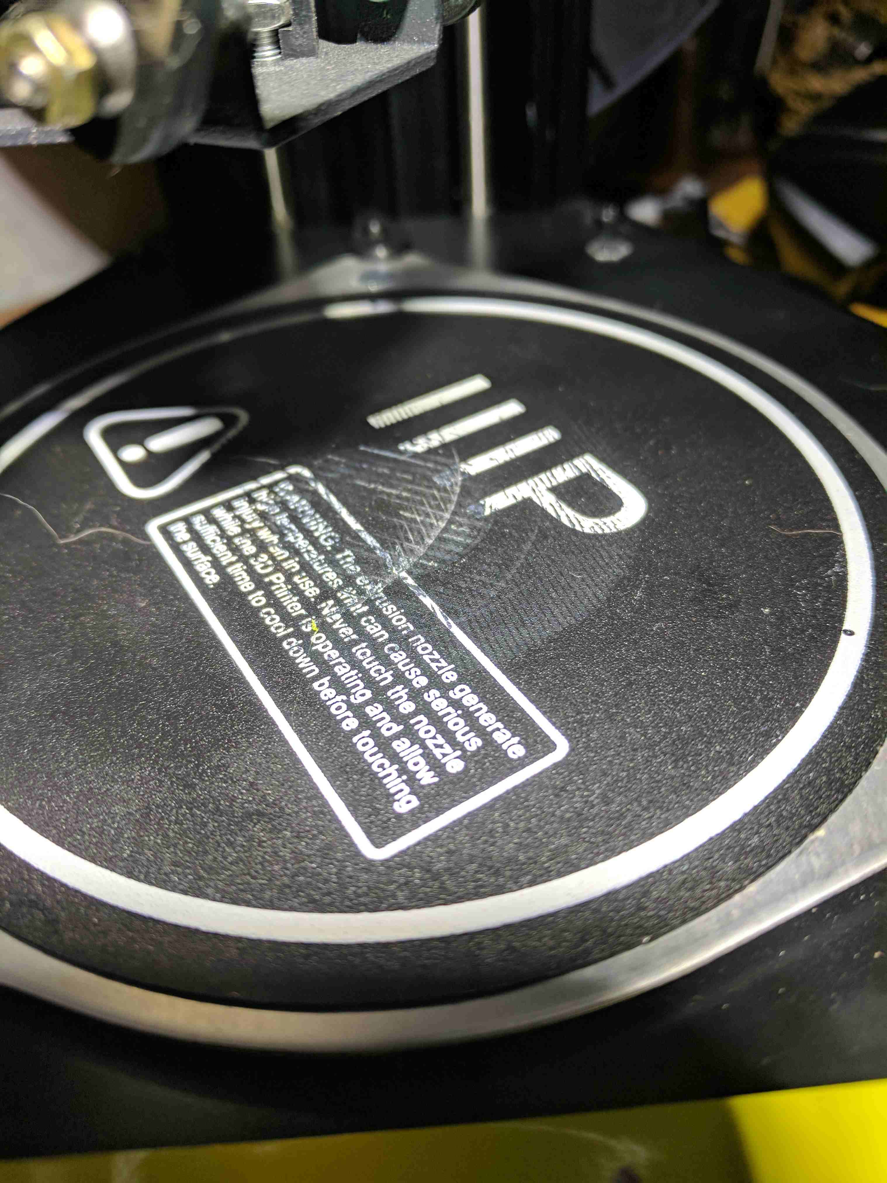
The auto bed level sensing is great, though each time it touches down it leaves a small amount of plastic stuck to the bed. I have been removing that between prints, if I didn't I imagine it would throw off the level sensing and cause problems.

While tweaking the tools (described below) to match this machine I generated a few files that directed the print head outside of the workable area, crashing it into parts of the machine that it really shouldn't be touching. I'm amazed that everything seems to be working fine now (I'm sure there's some extra wear on the timing belts and pulleys). I feel like the printer firmware should enforce limits on the print head movement to protect itself.

Tools used

Setting up the printer was not trivial, mainly because I didn't want to use the provided Windows executable. Since I've never had a 3D printer before, I had to decide which tools to use. There are roughly three steps to making something new with a 3D printer:

First you need to design your awesome new object. This is done with a CAD (Computer Aided Design) tool, and the result is a file that describes the geometry of the object. You can also download pre-made objects from sites like Thingiverse. It could be as simple as a file that specifies that it is a cube 1cm on a side. For this I used OpenSCAD.

Second the geometry needs to be turned into a sequence of operations for the printer to use to lay down the plastic needed to make the object. This is called slicing, and is where decisions like how the inside should be filled, how thick each layer should be, and whether some additional support or build platform should be added are made, among many others. The result of this step is almost always a sequence of primitive machine operations called G-code. I used Cura to handle this step.

Finally the G-code needs to be sent to the printer. The Mini Delta has three options here: you can transfer the file with an SD card, you can upload the file using a web interface exposed over WiFi, or you can send the instructions over USB. I used the SD card for the first few prints, tried to get the web interface to work ¹, and finally settled on using the USB interface. The USB interface uses one of the standard serial over USB protocols, but you can't just cat the G-code file over the serial port, there is a bit more to it. I found that Octoprint worked well for this.

OpenSCAD

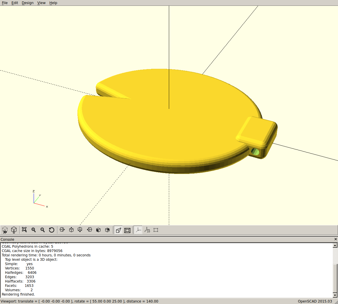
OpenSCAD is not for everyone, it trades constraint based modeling for programmatic control over the model ². As such it's more of a programmer's tool than a modeling tool. But it is fine for making some objects to print quickly. And I already knew how to use it because it's also what I've used in the past to model objects for laser cutting. Below is a screen shot of the zipper pull rendered in OpenSCAD.

You can find some of the OpenSCAD files I've made on Thingiverse.

Eventually I think I'll be using Solvespace for all my mechanical CAD work. It is a full parametric modeler, which is a very powerful way to create objects.

Cura

I selected Cura mainly because it's what Monoprice shipped on the SD card. First I created a custom printer. This is largely based on the CURA_CONFIG.ini file supplied with the printer on the SD card. But that file is for an older version of Cura that is also supplied on the SD card (as a Windows executable). So some changes had to be made. Unfortunately I wasn't able to find a way of writing a config file and importing it into Cura; I had to enter the printer config manually in the GUI. Below is the resulting configuration file that Cura saves as ~/.local/share/cura/master/definition_changes/Custom+FDM+printer_settings.inst.cfg.

[general]
version = 2
name = Custom FDM printer_settings
definition = custom

[metadata]
type = definition_changes
setting_version = 1

[values]
gantry_height = 0
machine_center_is_zero = True
machine_depth = 120
machine_end_gcode = ;End GCode
        M104 S0                      ;extruder heater off
        M140 S0                      ;heated bed heater off (if you have it)
        G91                          ;relative positioning
        G1 E-1 F300                  ;retract the filament a bit before lifting the nozzle, to release some of the pressure
        G1 Z+0.5 E-5 X-20 Y-20 F4800 ;move Z up a bit and retract filament even more
        G28 X0 Y0                    ;move X/Y to min endstops, so the head is out of the way
        M84                          ;steppers off
        G90                          ;absolute positioning
machine_head_with_fans_polygon = [[0, 0], [0, 0], [0, 0], [0, 0]]
machine_heated_bed = True
machine_height = 120
machine_shape = elliptic
machine_start_gcode = ;Sliced at: {day} {date} {time}
        ;Basic settings: Layer height: {layer_height} Walls: {wall_thickness} Fill: {infill_sparse_density}
        ;Print time: {print_time}
        ;Filament used: {filament_amount}m {filament_weight}g
        ;Filament cost: {filament_cost}

        G21            ;metric values
        G90            ;absolute positioning
        M82            ;set extruder to absolute mode
        M107           ;start with the fan off
        G28            ;Home
        G29 C-0.8 Z0.3 ;Auto level print platform
        G1 Z15.0 F4800 ;move the platform down 15mm
        G92 E0         ;zero the extruded length
        G1 F200 E3     ;extrude 3mm of feed stock
        G92 E0         ;zero the extruded length again
        G1 F4800

machine_width = 120
material_diameter = 1.75

Then I created a custom profile based on the draft profile and set the build plate adhesion type to "Raft", with an extra margin of 5mm. I found that without the raft it was extremely difficult to remove the prints. The raft also seems to protect the build plate a bit (the printing on the build plate sticks to the bottom of the print a bit). This results in a configuration file saved as ~/.local/share/cura/master/quality/custom_draft+quality+pla.inst.cfg. Cura does provide an export/import option for profiles, but it generates a ZIP file with a bunch of dummy profiles for up to eight extruders, not a simple text description like I was expecting. It seems easier to handle this step in the GUI as well.

[general]
version = 2
name = Draft Quality PLA
definition = fdmprinter

[metadata]
type = quality_changes
quality_type = draft
setting_version = 1

[values]
adhesion_type = raft
raft_margin = 5

Fortunately it is possible to easily import a filament description. Below is the material description file that I created for Cura.

<?xml version='1.0' encoding='utf-8'?>
<fdmmaterial version="1.3" xmlns="http://www.ultimaker.com/material">
  <metadata>
    <name>
      <brand>Shaxon</brand>
      <material>PLA</material>
      <color>Yellow</color>
      <label>yellow</label>
    </name>
    <setting_version>1</setting_version>
    <GUID>ea2fff89-1826-406f-bab0-4e612f2e5e20</GUID>
    <version>1</version>
    <color_code>#f4f442</color_code>
    <description></description>
    <adhesion_info></adhesion_info>
    <compatible>True</compatible>
  </metadata>
  <properties>
    <density>1.25</density>
    <diameter>1.75</diameter>
  </properties>
  <settings>
    <setting key="print temperature">190.0</setting>
    <setting key="heated bed temperature">70.0</setting>
    <setting key="retraction amount">4.0</setting>
    <setting key="retraction speed">80.0</setting>
    <setting key="standby temperature">150.0</setting>
    <setting key="print cooling">100.0</setting>
  </settings>
</fdmmaterial>

USB connection

The generic Linux usb serial driver doesn't yet know about the USB VID:PID pair for this printer, so in order to connect you need to provide it with them. My solution was to create a simple pair of UDEV rules.

#
# Add USB VID/PID for Monopride Mini Delta
#
ACTION=="add", SUBSYSTEM=="usb", ATTR{idVendor}=="cfce", ATTR{idProduct}=="0300", RUN+="/usr/bin/modprobe usbserial", RUN+="/bin/sh -c 'echo $attr{idVendor} $attr{idProduct} > /sys/bus/usb-serial/drivers/generic/new_id'"

#
# Construct a symlink to the TTY generated for the printer.
#
SUBSYSTEM=="tty", ATTRS{idVendor}=="cfce", ATTRS{idProduct}=="0300", SYMLINK+="monoprice_mini_delta"

I saved this as /etc/udev/rules.d/51-monoprice-mini-delta.rules, reloaded UDEV's rule database with sudo udevadm control --reload, and finally unplugged and plugged back in the printer USB cable. That gave me a handy symlink (/dev/monoprice_mini_delta) to use. To test that it worked I used screen to open the serial device (screen /dev/monoprice_mini_delta 115200) and sent a few G-code commands to the printer. In particular I sent G28 to home the axes, and M115 to get the machine information. For me M115 returns:

NAME. Malyan
VER: 3.7
MODEL: M300
HW: HG01
BUILD: Jun 26 2017 19:04:37

If you've never used screen, you can exit with Ctrl-A followed by '\'.

Octoprint

Setting up Octoprint on Arch Linux (my preferred desktop distribution) is pretty easy if you're familiar with the AUR. The package to install is octoprint-venv. And once installed you can enable and start the service with:

sudo systemctl enable octoprint.service
sudo systemctl start octoprint.service

Be warned: this runs Octoprint as root, probably not the best decision security-wise. By default Octoprint will start a web server listening to just the local machine on port 5000. So navigate over to http://localhost:5000 and you should be greeted with a nice GUI. The first thing to do is to connect to the printer. Use /dev/monoprice_mini_delta for the serial port, and 115200 for the baud rate. Once connected, go to the Control tab and try something safe, like turning the fan on and off.

The Octoprint GUI is pretty self-explanatory at this point; you can upload G-code files and print them. You also have a number of options for monitoring the print job, including graphs of bed and extruder temperature, visualization of the G-code instructions sent to the printer, and a raw stream of instructions.

The Control tab is also a lot of fun, but be careful, the Mini Delta's firmware doesn't prevent you from running the print head into the edge of the frame or down into the print bed. So make small moves until you have a good understanding of the machine.

I have been working on a game recently, and I ran into some interesting math along the way. I wanted an explosion animation that started out fast, and as it got larger it would get slower. Below you can click, drag or swipe to create the explosions I ended up building.

For simplicity, I am rendering the explosion as a ring, with expanding inner and outer radii. I wanted the rate of expansion of the two radii to start fast and end slow, but this could just as easily be applied to a collection of particles. One possible formula for velocity would be a linear ramp, changing from the initial to the final velocity in equal steps over the animation. That is, a constant change in velocity.

\[\frac{dV(t)}{dt} = \frac{V_T - V_0}{T}\]

But that didn't have the effect I was looking for; I wanted the leading edge of the ring to be moving really quickly and to slow down really quickly. And as it was near the end of the animation, moving more slowly, I wanted it to be slowing down more slowly as well. I wanted the change in velocity to be proportional to the current velocity.

\[ \begin{equation}\label{eqn:exponential_decay} \frac{dV(t)}{dt} = -\lambda V(t) \end{equation} \]

This differential equation, known as an Exponential Decay, is conventionally written with a negative sign so that the proportionality constant, \(\lambda\), will be positive. When \(\lambda\) is positive it continually subtracts a proportion of the velocity from itself, so when the velocity is large, the portion subtracted will be large, and when the velocity is small, the portion subtracted will be small. For completeness we'll also need a differential equation that relates position and velocity.

\[ \begin{equation}\label{eqn:position_diffeq} \frac{dX(t)}{dt} = V(t) \end{equation} \]

The combination of \(\eqref{eqn:exponential_decay}\) and \(\eqref{eqn:position_diffeq}\) is a system of differential equations; it says that the change in something's velocity (in our case the two ring radii) at some time will be proportional to the thing's velocity at that time. It also says that the change in the thing's position at some time is the thing's velocity. You can use these equations exactly as they are, via numeric integration. You iteratively update the velocity and position of the value you are simulating. The simplest way to do the update would be with the Euler method. You would select a small increment in time (a timestep) and move the simulation forward by that amount of time over and over again. For every timestep you update velocity by evaluating \(\eqref{eqn:exponential_decay}\), and then position by evaluating \(\eqref{eqn:position_diffeq}\). But if you want to know the position or velocity at a specific time you'll need to rerun the simulation from the beginning to get it, which could be very costly if you have selected a small timestep, which you would have to do to ensure an accurate simulation. Alternatively you could store all previous steps of the simulation, which would take a lot of memory. Either way, what values should you use for \(\lambda\) and the initial position and velocity? A better approach (at least for my needs) is to solve this differential equation analytically, and use the result to pick initial values and to evaluate position and velocity at arbitrary times.

Here is another version of the same expanding ring, rendered using the awesome online calculator Desmos. You can manually control the time slider (if you can grab it) to get a feel for how the two exponentials control the inner and outer radii of the ring.

So where's the interesting math? It turns out that picking the initial position, velocity, and \(\lambda\) values to get a good-looking explosion takes some care. For one thing, I wanted to make the final positions of the two exponenitals that control the inner and outer radii equal. I could have done that by trial an error, maybe, but there's a better way. In this post I'll go through solving \(\eqref{eqn:exponential_decay}\) and \(\eqref{eqn:position_diffeq}\) for a number of different parameters. We'll want an equation that can tell us the radius at a given time in the simulation. We'll also want to be able to compute initial velocity given some more intuitive parameters that make specifying the explosion simpler. In this case, it turns out to be easier to specify the final velocity, duration of explosion, and amount that the ring should expand. Given these, the initial velocity and \(\lambda\) are completely defined.

Velocity

The first step will be to solve \(\eqref{eqn:exponential_decay}\) so that we have an equation for velocity at an arbitrary time. This is a pretty simple differential equation, and we can solve it directly by integration.

The result is the solution for velocity at any time \(t\).

\[ \begin{equation}\label{eqn:velocity} V(t) = V_0 e^{-\lambda t} \end{equation} \]

Nothing too surprising here; this tells us how a value changes over time if it is continually being acted on in proportion to itself. Here is the same function written in Dart¹. This is one method from a class called ExponentialRate that I am using to model this system of differential equations in the game. The complete source for ExponentialRate can be found here.

///
/// Return the rate of change of the value at a given time.
///
/// Time can be negative, positive, or zero, it should also be able to be
/// positive or negative infinity, but I haven't verified that Dart's exp
/// function correctly handles those cases.
///
double rate(double time) => initial_rate * exp(-lambda * time);

Position

Next we want to know about the position over time, both so that we can query it for animations and so that we can solve the equation for our initial velocity. Now that we have \(\eqref{eqn:velocity}\), which is an equation for \(V(t)\), we can substitute it into \(\eqref{eqn:position_diffeq}\), our definition of position. This gives us a differential equation that we can solve.

The result is an explicit equation for \(X(t)\).

\[ \begin{equation}\label{eqn:position} X(t) = X_0 + \frac{1}{-\lambda} (V_0 e^{-\lambda t} - V_0) \end{equation} \]

Below you can experiment with \(\eqref{eqn:velocity}\) and \(\eqref{eqn:position}\), try changing \(X_0\), \(V_0\), \(\lambda\), and the total time of the simulation. \(V_0\) is controlled by manipulating the tangent line to the graph at the origin.

I noticed that the first term (\(V_0 e^{-\lambda t}\)) is just \(\eqref{eqn:velocity}\), so I used that in its place.

\[ \begin{equation}\label{eqn:position_from_rate} X(t) = X_0 + \frac{1}{-\lambda}(V(t) - V_0) \end{equation} \]

There is something very pleasing about this equation; the change in position is proportional to the change in velocity. But this form of the equation has some issues. One thing to note about this solution is that it doesn't work if \(\lambda\) is equal to zero. Fortunately \(\eqref{eqn:exponential_decay}\) then becomes trivial (\(\frac{dV(t)}{dt} = 0\)), and the solutions are \(V(t) = V_0\) and \(X(t) = X_0 + V_0 t\). However, when I thought about this more, I realized that this substitution of \(\eqref{eqn:velocity}\) had hidden a numerical issue in the implementation as well. If we start back with \(\eqref{eqn:position}\) and rearrange a little by factoring out \(V_0\) and moving \(\frac{1}{-\lambda}\) in we can see more clearly what the problem is.

\[X(t) = X_0 + V_0 \frac{e^{-\lambda t} - 1}{-\lambda}\]

The right term numerator is \(e^{-\lambda t} - 1\), which, for values of \(-\lambda t\) close to zero, can lead to Loss of Significance because we are subtracting two numbers that are nearly identical (\(e^0 = 1\)). It wasn't clear at first to me how to handle this; in C/C++ I would have used expm1 and then used the trivial solutions for \(\eqref{eqn:exponential_decay}\) and \(\eqref{eqn:position_diffeq}\) when \(\lambda\) was zero, but there would still be a possible problem with the division when \(\lambda\) is very close to zero because both numerator and denominator would be approaching zero. In hopes that I could come up with an alternate representation that would work for all values of \(\lambda\) and \(t\), I started to work with the infinite sum representation of the exponential function.

\[\def\exp_sum#1#2{\sum_{k=#1}^{\infty} \frac{#2^k}{k!}}\]

\[e^x = \exp_sum{0}{x}\]

I used this sum in place of the exponential in \(\eqref{eqn:position}\).

\[X(t) = X_0 + \frac{V_0}{-\lambda} (\exp_sum{0}{(-\lambda t)} - 1)\]

The first term in the sum is just one.

\[e^{-\lambda t} = 1 + \exp_sum{1}{(-\lambda t)}\]

That one cancels out the subtraction by one, leaving all of the remaining terms from \(\numrange{1}{\infty}\). All of those terms have at least one \(-\lambda\) in them, so I was able to divide the sum by \(-\lambda\), canceling out one of the \(-\lambda\) factors in each term. The result had no divisions by \(-\lambda\). Nice.

\[X(t) = X_0 + V_0 (\sum_{k=1}^{\infty} \frac{-\lambda^{k-1} t^k}{k!})\]

Then I saw that I could pull a \(t\) out of the sum as well. And I could shift the sum index (\(k\)) by one, so that the sum started at zero again.

\[X(t) = X_0 + V_0 t (\sum_{k=0}^{\infty} \frac{(-\lambda t)^k}{(k + 1)!})\]

The sum now looked so much like an exponential by itself that I was distracted into thinking that I could do something to recover a simple exponential form, with some additional damping factor (accounting for the \(+1\) in the factorial), that didn't have the division by zero problem that the original version had. Eventually I realized that the pulling out of \(t\) was the crucial piece that I had missed at first. I went back to \(\eqref{eqn:position}\) to see what would happen when I took a \(t\) out of the second factor.

\[ \begin{equation}\label{eqn:position_with_hex} X(t) = X_0 + V_0 t \frac{e^{-\lambda t} - 1}{-\lambda t} \end{equation} \]

I had to put a \(t\) in the denominator, which nicely turns the problematic portion into a one variable problem. No longer did I have to treat \(-\lambda\) and \(t\) as separate variables; I could just lump them together and work on solving \(\frac{e^x-1}{x}\), which at this point I feel like needs a name. If anyone knows of a name for this particular function² I would be interested, for now I'm calling it a hexponential, or \(hex(x)\), short for "half exponential" because the derivative at zero is one half instead of one, but otherwise it looks like an exponential.

\[hex(x) := \frac{e^x - 1}{x} = \sum_{k=0}^{\infty} \frac{x^k}{(k + 1)!}\]

Hex is well behaved at the origin, even with the division by zero, because the division is in some sense just an artifact of writing the function down in a Closed Form. We can use the sum representation to compute it around zero nicely. We can also see this by using L'Hôpital's rule to compute the limit of the closed form of hex. Here is the resulting version of \(\eqref{eqn:position_with_hex}\) written in Dart.

///
/// Return the value at a given time.
///
/// Time can be negative, positive, or zero, it should also be able to be
/// positive or negative infinity, but I haven't verified that Dart's exp
/// function correctly handles those cases.
///
double value(double time)
{
    //
    // This version of hex maintains about 14 digits of precision, not full
    // machine precision (~16 digits for doubles).
    //
    double hex(double x)
    {
        //
        // A threshold of 10^-2 seems like a good compromise.  The smaller
        // the threshold is, the fewer terms we need to use to accurately
        // evaluate hex.  But smaller thresholds increase the loss of
        // significance when using the exponential form below.  The
        // truncation error introduced by a threshold of 10^-2 is O(x^6),
        // or on the order of 1e-12.  In fact, the first term that we lose
        // from the sum is x^6/6!, or 10^-12/720, or 1.38e-15, so our
        // truncation error is closer to 1e-15.
        //
        if (x.abs() < 1e-2)
            return 1 + (1 + (1 + (1 + x / 5) * x / 4) * x / 3) * x / 2;

        //
        // The worst case loss of significance from the subtraction below
        // will be when x = 10^-2.
        //
        // log2(1-(1/e^(10^-2))) ~ -6.6
        //
        // So we can expect to loose 7 bits of precision, from our doubles
        // 53 bit mantissa.  Or ~2 digits from our ~16 digits of precision.
        //
        return (exp(x) - 1) / x;
    }

    return initial_value + initial_rate * time * hex(-lambda * time);
}

Lambda

We now have our solutions for \(\eqref{eqn:exponential_decay}\) and \(\eqref{eqn:position_diffeq}\), but we're still stuck specifying \(X_0\), \(V_0\), \(\lambda\), and \(T\) (the total time of the simulation). Instead, we would like to be specifying \(X_0\), \(X_T\), \(V_T\), and \(T\), where

\[ \begin{align*} X_T &:= X(T)\\ V_T &:= V(T). \end{align*} \]

In other words, we need to come up with equations that give us \(V_0\) and \(\lambda\) in terms of \(X_0\), \(X_T\), \(V_T\), and \(T\).

We can use \(\eqref{eqn:velocity}\), the solution for our velocity at a given time, to compute \(\lambda\) if we know \(V_0\), \(V_T\), and \(T\). This can then be substituted into \(\eqref{eqn:position}\) which gives us an equation relating \(X_0\), \(X_T\), \(V_0\), \(V_T\), and \(T\). We can then solve that equation for \(V_0\).

\[ \begin{equation}\label{eqn:lambda} \lambda = -\frac{log(\frac{V_T}{V_0})}{T} \end{equation} \]

We will need to use this equation once we've solved \(\eqref{eqn:position}\) for \(V_0\) to compute \(\lambda\). Again, we can write \(\eqref{eqn:lambda}\) in Dart.

///
/// Compute the proportionality coefficient lambda given the start and end
/// rates as well as total time taken.
///
static double _lambda(double final_rate,
                      double initial_rate,
                      double total_time)
{
    //
    // If final_rate, or initial_rate is zero then the other must also be
    // zero.  This is because the only way to actually get to zero with an
    // exponential is to already be there.  And if you're there, there is
    // no way to leave.  In this case lambda should be zero, because our
    // rate is not changing.
    //
    assert((final_rate == 0.0) == (initial_rate == 0.0));

    if (final_rate == 0.0)
        return 0.0;

    //
    // Lambda is not a complex number, we are only interested in solving
    // for real values.  So final_rate and initial_rate must also have the
    // same sign.
    //
    assert((final_rate > 0.0) == (initial_rate > 0.0));

    return -log(final_rate / initial_rate) / total_time;
}

We can now substitute \(\eqref{eqn:lambda}\) into \(\eqref{eqn:position}\), giving us an equation for position that is parameterized by \(X_0\), \(V_0\), \(V_T\), and \(T\).

\[ \begin{equation}\label{eqn:position_no_lambda} X(t) = X_0 + \frac{T}{log(\frac{V_T}{V_0})} (V_0 e^{\frac{log(\frac{V_T}{V_0})}{T} t} - V_0) \end{equation} \]

We can play with this function in Desmos as well, but we still don't get to specify the final position of the animation (\(X_T\)).

You'll probably notice that \(V_0\) and \(V_T\) have to have the same sign. If they do not then desmos doesn't show a graph at all. This is because \(\eqref{eqn:lambda}\) takes the logarithm of their ratio, and as long as \(V_0\) and \(V_T\) have the same sign their ratio is positive. The logarithm for real numbers is not defined for negative numbers. So Desmos (and the Dart implementation above) give up. But if we were to use the complex exponential and logarithm then there is actually a solution when \(V_0\) and \(V_T\) have different signs. The solution ends up being a combination of sine, cosine and exponential functions. The sine and cosine allow for the change in sign of the rate. I touched on this briefly at the end of my 2D Rotation post. It is never the case in the game I'm writing that I want the initial and final velocities to have different signs, so I opted to keep the solution real. I could imagine an explosion animation that contracts at the end, but that wasn't what I was going for visually.

Initial Velocity

We now have \(\eqref{eqn:position}\) that tells us \(X_T\) given \(X_0\), \(V_0\), \(\lambda\), and \(T\). And we just found \(\eqref{eqn:lambda}\), an equation for \(\lambda\). Then we substituted \(\eqref{eqn:lambda}\) into \(\eqref{eqn:position}\) to get \(\eqref{eqn:position_no_lambda}\). Now we'll solve the result for \(V_0\). This is where the math got interesting; I had never encountered the Lambert W function before. And it turns out that solving for \(V_0\) will need it. To apply it we need to get one side of this equation to look like \(f(V_0) e^{f(V_0)}\), and the other side to not have \(V_0\) in it. Because it will make the remaining math easier to follow I'm going define \(\Delta X\) here.

\[\Delta X := X_T - X_0\]

We now have an equation that relates all of our coefficients (\(X_0, X_T, V_0, V_T\), and \(T\)); We just have to solve it for \(V_0\).

\[ \begin{equation}\label{eqn:initial_velocity_symetric} -T \frac{V_T}{\Delta X} e^{-T \frac{V_T}{\Delta X}} = -T \frac{V_0}{\Delta X} e^{-T \frac{V_0}{\Delta X}} \end{equation} \]

Now that the right hand side is in the correct form \(f(V_0) = -T \frac{V_0}{\Delta X}\), we can apply W to both sides. You might notice that the left hand side is also in the same form, it is \(f(V_T) = -T \frac{V_T}{\Delta X}\). More about that later.

\[ W(-T \frac{V_T}{\Delta X} e^{-T \frac{V_T}{\Delta X}}) = -T \frac{V_0}{\Delta X} \]

And finally, multiply both sides by \(-\frac{\Delta X}{T}\) to solve for \(V_0\).

\[ V_0 = -W(-T \frac{V_T}{\Delta X} e^{-T \frac{V_T}{\Delta X}}) \frac{\Delta X}{T} \]

This is a lot to look at, but it has some repetition that we can factor out, making it easier to understand; substitute \(A = -T \frac{V_T}{\Delta X}\).

\[ \begin{equation}\label{eqn:initial_velocity} V_0 = V_T \frac{W(A e^A)}{A} \end{equation} \]

I wanted to add a Desmos graph here where you could play with the new set of parameters, but Desmos doesn't currently support the Lambert W function, which makes it pretty hard to evaluate the above equation. It could be approximated with a lot of work, but this post has taken long enough to write already.

But we can get an idea for the sort of solutions that the Lambert W function would return. Below is a graph of \(f(x) = xe^x\) that shows that for any value of \(x_1 < 0\) other than \(x_1 = -1\) there is another value \(x_2 \neq x_1\) such that \(f(x_1) = f(x_2)\). In other words, if \(x\) is less than zero, and not equal to negative one, then the inverse of \(f(x)\) has two values. That other value can be computed using one of the two branches of the Lambert W function.

I'd like to return briefly to the interesting symmetry of \(\eqref{eqn:initial_velocity_symetric}\), it was of the form:

\[X e^X = Y e^Y\]

where

\[ \begin{align*} X &:= f(V_T) = -T \frac{V_T}{\Delta X}\\ Y &:= f(V_0) = -T \frac{V_0}{\Delta X}. \end{align*} \]

Our problem was that we were given \(Y\) and we needed to compute \(X\), more or less. It's probably obvious that there's a trivial solution to this problem; \(X = Y\). That makes both sides identical, and so obviously it's a solution to \(\eqref{eqn:initial_velocity_symetric}\), but we arrived at \(\eqref{eqn:initial_velocity_symetric}\) by manipulating \(\eqref{eqn:position}\). And \(\eqref{eqn:position}\) is not valid when \(V_T = V_0\) (because then \(\lambda\) is zero), and since \(X\) and \(Y\) are just \(f(V_T)\) and \(f(V_0)\), \(X = Y\) can't be a solution we're actually looking for. Fortunately, there is a second solution for all values of \(A\) other than \(-1\). When \(A = -1\) the initial rate is just the final rate.

///
/// Return the initial rate that will result in the given change in value
/// and rate, over the specified total time.
///
/// delta_value in [        0 .. infinity)
/// final_rate  in (-infinity .. infinity)
/// total_time  in [        0 .. infinity)
///
static double _initial_rate(double delta_value,
                            double final_rate,
                            double total_time)
{
    ///
    /// If delta_value is zero, then final_rate must also be zero.  It is
    /// not possible to have zero change in value with a non-zero
    /// final_rate because the exponential is monotonic.
    ///
    assert(delta_value != 0.0 || final_rate == 0.0);

    ///
    /// Since we're not expected to change the value at all, and final_rate
    /// is zero, _initial_rate should also be zero.
    ///
    if (delta_value == 0.0)
        return 0.0;

    ///
    /// If total_time is zero, then delta_value must also be zero.  If
    /// delta_value were not zero we would have to somehow give two
    /// different values for the same instant in time.
    ///
    assert(total_time != 0.0 || delta_value == 0.0);

    ///
    /// If total_time is zero then _initial_rate will match final_rate.
    ///
    if (total_time == 0.0)
        return final_rate;

    final double A = -total_time * final_rate / delta_value;

    if (A > -1.0)
        return W_negative_one(A * exp(A)) * final_rate / A;

    if (A < -1.0)
        return W_zero(A * exp(A)) * final_rate / A;

    return final_rate;
}

To evaluate the Lambert W function I wrote a version of the approximations found in Having Fun with Lambert W(x) Function. A post about that implementation might be a good idea. For now, the source can be found here.

Dimensional Analysis

It's a good idea to double check our work and make sure that the resulting equations make sense from a units perspective. Let's add units. First we'll figure out the units of \(\lambda\). We start with \(\eqref{eqn:lambda}\) and add units to the right side.

\[ \lambda = -\frac{log(\frac{V(t) \si{m s^{-1}}}{V_0 \si{m s^{-1}}})}{t \si{s}} \]

The units of velocity (\(\si{m s^{-1}}\)) cancel, leaving the numerator unitless. The denominator still has units of seconds, so lambda has units of inverse seconds, also known as Hertz, a unit of frequency.

The units for \(\eqref{eqn:velocity}\) are also simple.

\[V(t) = V_0 \si{m s^{-1}} e^{-\lambda \si{s^{-1}} t \si{s}}\]

The units of \(\lambda\) and \(t\) in the exponential cancel, leaving that unitless. The only remaining units are from \(V_0\), so \(V(t)\) has the same units, those of velocity.

Next we can check the units for \(\eqref{eqn:position_from_rate}\).

\[ X(t) \si{m} - X_0 \si{m} = \frac{1}{-\lambda \si{s^{-1}}} (V(t) \si{m s^{-1}} - V_0\si{m s^{-1}}) \]

We can cancel \(\si{s^{-1}}\) from numerator and denominator, leaving meters on both sides, giving the correct units for position.

Finally let's check \(\eqref{eqn:initial_velocity}\) - to do that we just have to show that \(A(t)\) is unitless.

\[A(t) = -t \si{s} \frac{V(t) \si{m s^{-1}}}{X(t) \si{m}}\]

Pretty easy to see that seconds and meters cancel out completely.

I'm hoping with this post to show one way that complex numbers come about and how they are a natural way of representing rotations in 2D. To do this I will introduce a small amount of Clifford algebra and some infinite series expansions. A benefit of understanding rotations in this way will be that it generalizes to arbitrary dimensions, though you probably only care about the two and three dimensional cases.

A friend of mine recently asked me about 2D rotations. He had started with a 2x2 rotation matrix:

\[ \left( \begin{array}{cr} cos(\theta) & -sin(\theta)\\ sin(\theta) & cos(\theta)\\ \end{array} \right) \left( \begin{array}{c} x\\ y\\ \end{array} \right) = \left( \begin{array}{c} cos(\theta) x - sin(\theta) y\\ sin(\theta) x + cos(\theta) y\\ \end{array} \right) \]

After playing with it for a while he concluded that the second row of the matrix was redundant and you could just store the first row, or really any row or column. This reminded him of something I had said a while back about using complex numbers to represent rotations. This prompted me to write a first version of this post as an email in response. Then he wrote again saying that it seemed like the two component thing was the result of \(e^{i\theta}\). So I have added a section on the exponential map and Taylor series.

Complex Numbers

First let's start with a bit of a review of complex numbers. You've probably been introduced to them at some point as a number with two components, a real portion and an imaginary portion, where the imaginary portion is signified by having a lower case \(i\) associated with it.

\[(a + b i)\]

And they were probably being used to fill in a gap when someone tried to take the square root of a negative number. Probably it was right around when you learned the quadratic formula. Some people are introduced to complex numbers when they start playing with fractals; the Mandelbrot set, Julia sets, and others are defined in the complex plane. The complex plane is what you get if you treat the real and imaginary parts of a complex number as the \(x\) and \(y\) components of a 2D vector. A lot of neat results come from that mapping. Later I'll show a different way to associate the components of a complex number with the \(x\) and \(y\) components of a 2D vector, but first, let's remember what happens when you multiply two complex numbers together.

\[(a_1 + b_1 i) (a_2 + b_2 i)\]

You probably remember FOIL (First Outer Inner Last) which tells you how to go about doing this multiplication. First multiple the a's together, then the outer elements \((a_1 \text{and} b_2 i)\), then the inner elements \((b_1 i \text{and} a_2)\), and finally the last elements, the b's.

\[(a_1 a_2) + (a_1 b_2 i) + (b_1 i a_2) + (b_1 i b_2 i)\]

With complex numbers we're free to move the i's around inside each product, so we'll move them to the end of each one, and outside of the parentheses.

\[(a_1 a_2) + (a_1 b_2) i + (b_1 a_2) i + (b_1 b_2) i i\]

The \(i i\) that we get from the multiplication of the two imaginary components \((b_1 \text{and} b_2)\) of the two complex numbers could also be written \(i^2\). The whole reason for inventing \(i\) was to provide an answer to the question of what \(x\) is in the following.

\[x = \sqrt{-1}\]

So, \(i^2 = -1\), and thus the result of multiplying two imaginary components of a complex number together is a real number, just one that has the opposite sign than it would otherwise. So, taking this into account and merging the two terms in the middle that each have a single \(i\) in them we can simplify the result of multiplying two complex numbers down to the following.

\[(a_1 a_2) + (a_1 b_2 + b_1 a_2) i - (b_1 b_2)\]

Finally, moving the imaginary portion to the end we get:

\[(a_1 a_2 - b_1 b_2) + (a_1 b_2 + b_1 a_2) i\]

Which is another complex number \((a_3 + b_3 i)\) where \(a_3\) and \(b_3\) are defined as:

\[\begin{align*} a_3 &= a_1 a_2 - b_1 b_2 \\ b_3 &= a_1 b_2 + b_1 b_2 \end{align*}\]

With that basic review of complex numbers, let's move on to talk about the Clifford algebra.

Clifford Algebra

Above we had said that you could make a 2D plane by associating the real and imaginary components of a complex number with the \(x\) and \(y\) elements of a 2D vector. But we didn't really talk about what that meant or how you could distinguish an \(x\) component from a \(y\) component. There has been an enormous amount written about this subject, and I highly recommend Geometrical Vectors by Gabriel Weinreich. But for now, I'm going to introduce two new things, sort of like \(i\) from the complex numbers, called \(\mathbf{e_1}\) and \(\mathbf{e_2}\). And we will use them to distinguish between the two components of a 2D vector. So, our vectors will look like this. \((x \mathbf{e_1} + y \mathbf{e_2})\) These things, we'll call them bases, have a few properties: a base times itself equals one, and swapping the position of two bases in a term negates the term.

\[ \mathbf{e_i e_i} = 1\\ \mathbf{e_i e_j} = - \mathbf{e_j e_i} \]

These vectors behave just like you would expect a vector to behave. You can add and subtract them.

\[ (x_1 \mathbf{e_1} + y_1 \mathbf{e_2}) + (x_2 \mathbf{e_1} + y_2 \mathbf{e_2}) = ((x_1 + x_2) \mathbf{e_1} + (y_1 + y_2) \mathbf{e_2}) \]

And you can multiply them by scalars.

\[ c (x_1 \mathbf{e_1} + y_1 \mathbf{e_2}) = (c x_1 \mathbf{e_1} + c y_1 \mathbf{e_2}) \]

But they also have another interesting trick, if we multiply two of these vectors together we get an interesting new object.

\[(x_1 \mathbf{e_1} + y_1 \mathbf{e_2}) (x_2 \mathbf{e_1} + y_2 \mathbf{e_2})\]

using FOIL you get

\[(x_1 x_2) \mathbf{e_1 e_1} + (x_1 y_2) \mathbf{e_1 e_2} + (y_1 x_2) \mathbf{e_2 e_1} + (y_1 y_2) \mathbf{e_2 e_2}\]

Since \(\mathbf{e_1 e_1} = 1\) and \(\mathbf{e_2 e_2} = 1\) the first and last terms turn into scalars and you get

\[(x_1 x_2) + (x_1 y_2) \mathbf{e_1 e_2} + (y_1 x_2) \mathbf{e_2 e_1} + (y_1 y_2)\]

Now, the middle two terms can be combined by swapping the \(\mathbf{e_2 e_1}\) in the second term to be \(\mathbf{e_1 e_2}\) and negating the whole term. So the result is

\[(x_1 x_2) + (x_1 y_2 - y_1 x_2) \mathbf{e_1 e_2} + (y_1 y_2)\]

Finally, grouping the first and last term together you get

\[(x_1 x_2 + y_1 y_2) + (x_1 y_2 - y_1 x_2) \mathbf{e_1 e_2}\]

We see that the first term is just the dot product of the two vectors, and the second term is just the 2D cross product ¹ times something weird, this \(\mathbf{e_1 e_2}\) term. So we've got some new odd object here: a scalar plus a scalar times a strange pair of bases. If we replace the dot and cross product values with the letters \(a\) and \(b\) we have \(a + b \mathbf{e_1 e_2}\).

As you may know, the dot product of two vectors is equal to the cosine of the angle between them times the length of each vector. Similarly, the length of the cross product of two vectors is equal to the sine of the angle between them times the length of each vector. These sines and cosines allow us to get back to rotation.

2D Rotation Revisited

Now what happens if we multiply one of our original vectors times one of these?

\[(x \mathbf{e_1} + y \mathbf{e_2}) (a + b \mathbf{e_1 e_2})\]

We get:

\[(a x) \mathbf{e_1} + (b x) \mathbf{e_1 e_1 e_2} + (a y) \mathbf{e_2} + (b y) \mathbf{e_2 e_1 e_2}\]

Which after simplification is:

\[(a x - b y) \mathbf{e_1} + (b x + a y) \mathbf{e_2}\]

Which looks a lot like a rotation matrix application. ² Especially when you remember that if the two vectors we started with are unit length then a and b are equal to the cos and sin of the angles between the two vectors. In which case we have:

\[a = cos(\theta)\\ b = sin(\theta)\]

and after substitution:

\[ \begin{align*} &(cos(\theta) x - sin(\theta) y) \mathbf{e_1} +\\ &(sin(\theta) x + cos(\theta) y) \mathbf{e_2} \end{align*} \]

Complex Numbers Revisited

You can probably see where this is going. Let's try multiplying two of these 'scalar plus scalar times base pairs' together.

\[ (a_1 + b_1 \mathbf{e_1 e_2}) (a_2 + b_2 \mathbf{e_1 e_2}) \]

Again, using FOIL we get:

\[ (a_1 a_2) + (a_1 b_2) \mathbf{e_1 e_2} + b_1 \mathbf{e_1 e_2} a_2 + b_1 \mathbf{e_1 e_2} b_2 \mathbf{e_1 e_2} \]

It is fine to move the scalars around, so let's clean this up:

\[ (a_1 a_2) + (a_1 b_2) \mathbf{e_1 e_2} + (a_2 b_1) \mathbf{e_1 e_2} + (b_1 b_2) \mathbf{e_1 e_2 e_1 e_2} \]

We can combine the two \(\mathbf{e_1 e_2}\) terms:

\[ (a_1 a_2) + (a_1 b_2 + a_2 b_1) \mathbf{e_1 e_2} + (b_1 b_2) \mathbf{e_1 e_2 e_1 e_2} \]

Next we deal with the \(\mathbf{e_1 e_2 e_1 e_2}\) term. If we swap the middle \(\mathbf{e_2 e_1}\) into \(\mathbf{e_1 e_2}\) and negate the whole thing we get \(-\mathbf{e_1 e_1 e_2 e_2}\). And since a base times itself is \(1\) we have \(-1 * 1\) or \(-1\). So, the last term can be replaced with \(-(b_1 b_2)\), causing the entire thing to turn into:

\[ \begin{align*} &(a_1 a_2 - b_1 b_2) +\\ &(a_1 b_2 + a_2 b_1) \mathbf{e_1 e_2} \end{align*} \]

And poof, we have another one of these scalar plus scalar times \(\mathbf{e_1 e_2}\) things. The fact that \(\mathbf{e_1 e_2 e_1 e_2} = -1\) should have given it away: \(\mathbf{e_1 e_2}\) could also be called \(i\) and these are complex numbers (or at least they behave like them, which in some sense means that they are them).

If complex numbers really do represent rotations in 2D then we would expect that there would be a way to combine two rotations that are represented by complex numbers, resulting in a single complex number that represents the combined rotation. And you are probably not surprised to learn that there is, and it is just complex multiplication (which we worked out above). To show this let's assume that \((a_1 + b_1 \mathbf{e_1 e_2})\) represents a rotation by \(\theta\) radians and \((a_2 + b_2 \mathbf{e_1 e_2})\) represents a rotation by \(\phi\) radians. So:

\[ a_1 = cos(\theta)\\ b_1 = sin(\theta)\\ a_2 = cos(\phi)\\ b_2 = sin(\phi) \]

If we rewrite the result of multiplying two complex numbers together and substitute these cosines and sines in we get:

\[ \begin{align*} &(cos(\theta) cos(\phi) - sin(\theta) sin(\phi)) +\\ &(cos(\theta) sin(\phi) + cos(\phi) sin(\theta)) \mathbf{e_1 e_2} \end{align*} \]

Now we have to remember (or re-derive, but this post is getting too long as it is) the sin and cos of the sum of angles formulas. They are, probably not surprisingly:

\[ \begin{align*} cos(\theta + \phi) &= cos(\theta) cos(\phi) - sin(\theta) sin(\phi)\\ sin(\theta + \phi) &= cos(\theta) sin(\phi) + cos(\phi) sin(\theta)\\ \end{align*} \]

And thus, we can rewrite the product of two complex numbers that represent rotations as:

\[cos(\theta + \phi) + sin(\theta + \phi) \mathbf{e_1 e_2}\]

And indeed, the product of two complex numbers that represent rotations, is itself a rotation, one that is the sum of the two independent rotations.

Exponential Map

The exponential map is a special function that is its own derivative. It is fascinating, and I recommend reading more about it. Here I'm just going to quickly show one fantastic result. I'll need to use the words Taylor Series and infinity, but I'm not going to justify them much. It can be thought of as an infinite sum of terms, or as the exponentiation \(e^x\).

\[exp(x) = e^x = \sum_{k=0}^{\infty} \frac{x^k}{k!}\]

This function is valid for all complex numbers, but we will limit the input to just the imaginary numbers (the imaginary portion of a complex number). To make the notation a little simpler I'll use \(i\) instead of \(\mathbf{e_1 e_2}\). I'll show that by doing this we effectively map an infinite line to the circle of radius one centered at the origin of the complex plane. Points on the line can be thought of as representing angles in radians. And every time we move \(2 \pi\) along the line we make one full loop around the circle. So, there are many points on the line that map to the same point on the circle. These all represent the same rotation.

\[exp(x i) = e^{x i} = \sum_{k=0}^{\infty} \frac{(x i)^k}{k!}\]

First, let's look at the \((x i)^k\) term. The first few terms in the infinite sum and the generalization for an arbitrary value of \(k\) are:

\[ \begin{align*} (x i)^0 &= x^0 = 1\\ (x i)^1 &= x^1 i = x i\\ (x i)^2 &= x^2 i i = -1 x^2\\ (x i)^3 &= x^3 i i i = -1 x^3 i\\ &\vdots\\ (x i)^k &= x^k i^k = \begin{cases} -1^{\frac{k}{2}} x^k & k\;\text{is even} \\[1ex] -1^{\frac{k-1}{2}} x^k i & k\;\text{is odd} \end{cases}\\ \end{align*} \]

If we group all of the even and all of the odd terms together we get:

\[ e^{x i} = \sum_{k=0,2,4...}^{\infty} \frac{-1^{\frac{k}{2}} x^k}{k!} + \sum_{k=1,3,5...}^{\infty} \frac{-1^{\frac{k-1}{2}} x^k}{k!}i \]

We can turn the sums back into simple sums from zero to infinity by transforming \(k\) in each of them. In the first one we can replace \(k\) with \(2k\), and in the second we can replace \(k\) with \(2k+1\). The result is:

\[ e^{x i} = \sum_{k=0}^{\infty} \frac{-1^k x^{2k}}{(2k)!} + \sum_{k=0}^{\infty} \frac{-1^k x^{2k+1}}{(2k+1)!}i \]

It turns out that the first sum is actually the Taylor series expansion for \(cos(x)\) and the second sum is the Taylor series expansion for \(sin(x)\). So this can be rewritten as:

\[ e^{x i} = cos(x) + sin(x) i \]

This beautiful result is known as Euler's formula.

Further Reading

• Universal Geometric Algebra

Mandelbrot is a javascript implementation of a simple mandelbrot set calculator.

//
// Set the pixel at location <x,y> in the image data to <r,g,b,a>.  The r, g,
// and b elements are the red, green, and blue color components.  The a element
// is the alpha, or transparency value.  The r, g, b, and a values can range
// from 0 to 255.
//
function set_pixel(image_data, x, y, r, g, b, a)
{
    // Compute the index into the pixel data.  Each pixel is represented by four
    // sequential values in the image_data.data array.
    index = (x + y * image_data.width) * 4;

    image_data.data[index + 0] = r;
    image_data.data[index + 1] = g;
    image_data.data[index + 2] = b;
    image_data.data[index + 3] = a;
}

//
// Compute the number of iterations required for a single orbit of the
// mandelbrot equation to escape from a circle of radius 2 centered at the
// origin of the complex plane.
//
function compute_escape_time(c_r, c_i, maximum_iterations)
{
    z_r = 0.0;
    z_i = 0.0;

    for (i = 0; i < maximum_iterations; i++)
    {
	//
	// Compute a single iteration of Z^2 + C.  Complex numbers are of the
	// form "real + imaginary * i", so to square them you end up computing:
	//
	// (real + imaginary * i) * (real + imaginary * i)
	// =
	// real * real + imaginary * imaginary * i^2 + 2 * real * imaginary * i
	// =
	// real * real - imaginary * imaginary + 2 * real * imaginary * i
	//
	// So the new real value is (real * real - imaginary * imaginary)
	// And the new imaginary value is (2 * real * imaginary)
	//
	// The reason the first + turns into a - is because i^2 is defined to be
	// equal to -1, that's what makes the numbers imaginary.
	//
	temp = (z_r * z_r) - (z_i * z_i) + c_r;
	z_i = (2.0 * z_r * z_i) + c_i;
	z_r = temp;

	// Check to see if the magnitude of the complex number is larger than
	// 2.  We check whether the squared magnitude is greater than 4 here to
	// avoid taking a square root, because square roots are slow.
	if (((z_r * z_r) + (z_i * z_i)) > 4.0)
	    return i;
    }

    // Return the maximum iterations value if we never escaped.
    return maximum_iterations;
}

//
// Draw a Mandelbrot set filling in a canvas specified by element_id.
//
function draw_mandelbrot(element_id)
{
    // Lookup the canvas and get a 2D rendering context from it.
    element = document.getElementById(element_id);
    context = element.getContext("2d");

    //
    // Construct an image data object to hold the pixels before they are
    // drawn to the screen.
    //
    image_data = context.createImageData(element.width,
					 element.height);

    //
    // Iterate over every pixel in the canvas and compute the escape time for
    // the corresponding point in the complex plane.
    //
    for (y = 0; y < image_data.height; y++)
    {
	for (x = 0; x < image_data.width; x++)
	{
	    //
	    // This scales the <x, y> values into a smaller range of the
	    // complex plane.  But it doesn't take into account the size of the
	    // canvas element.  So if the canvas element changes size, this will
	    // need to change as well.  This can be made automatic, but it would
	    // obcure the meaning for this example.  It would be a good
	    // experiment to change these values and try and make the result
	    // general.
	    //
	    iterations = compute_escape_time((x - 350.0) / 200.0,
					     (y - 250.0) / 200.0,
					     100);

	    //
	    // This is a simple use of the iteration count.  We are only looking
	    // at the bottom bit of the resulting escape time iterations.  This
	    // results in the zebra striping look.
	    //
	    if (iterations & 1)
		r = g = b = 255;
	    else
		r = g = b = 0;

	    //
	    // Write the computed color value to the image_data at the current
	    // location.
	    //
	    set_pixel(image_data, x, y, r, g, b, 255);
	}
    }

    // Finally, copy the resulting image to the canvas for display.
    context.putImageData(image_data, 0, 0);
}

Syntax highlighted with Prism.

This HOWTO describes the steps required to extract a portion of a large git repository into it's own separate repository.

I have found this useful numerous times because when I first started to use git I created a single repository for all of my personal projects. Since then I've come to appreciate having many smaller repositories. So whenever I want to open up some new chunk of code I use these steps to extract the history for just that chunk into a new repository and then publish that.

Setup

I always start by doing a fresh clone of the repository that I want to extract from, so that I know I'm not messing with my primary development environment. This has the added advantage that as long as you don't clone with --recursive, you won't have any submodules checked out. If you have submodules then the filter branch can get into trouble trouble.

git clone git://source.socialhacker.com/... temp_clone

Then just to make sure I'm not going to do something stupid, I remove the remote from the newly cloned repository.

cd temp_clone
git remote rm origin

Now we're ready to run git filter-branch. In particular, I run the subdirectory filter which replays all of your commits, only keeping changes to a given subdirectory. You need to add the --prune-empty option to cause filter-branch to not include empty commits.

git filter-branch \
    --prune-empty \
    --subdirectory-filter <directory> \
    -- \
    --all

Now, at this point I like to fix up the history a little. In particular I fix up the commit messages with the name and email address I've decided on. For a while I hadn't set these correctly and my early commits have something pretty useless. This will only work if you're the only committer to your repository. If you have multiple people committing, then this will wipe out their author names and email addresses from their commits.

git filter-branch \
    -f \
    --env-filter "export GIT_AUTHOR_NAME='Anton Staaf'; export GIT_AUTHOR_EMAIL='anton@socialhacker.com';" \
    HEAD

git filter-branch \
    -f \
    --env-filter "export GIT_COMMITTER_NAME='Anton Staaf'; export GIT_COMMITTER_EMAIL='anton@socialhacker.com';" \
    HEAD

The final step before you can push your new repository is to remove all of the old information about the commits that you no longer want to be visible. The first line below clears out the reflog, so that it doesn't maintain references to the old state of the repository. The second line does a garbage collection run on the repository. This will remove any objects that are no longer referenced.

git reflog expire --expire=now --all
git gc --aggressive --prune=now

At this point you can add a new remote and push your repository.